User:Xappppp
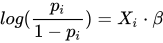
l o g ( p i
Logistic Regression Model
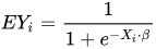
Model
i is the index for each individual observation, or in the other form.
Estimation
To estimate the parameter , we maximize the likelihood function:


where, are binary dependent variables, and this maximization procedure is done by numerical method such as Newton Raphson.

Odds Ratio
Let's set up a simple case: logistic model with one factorial factor ( level, which can be more level):
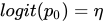

and the Odds Ratio of level-i over the base line level is

The confidence interval of OR is the exponential of confidence interval of .

In more than one factor case, this is this still the same, conditioning on other factors remain fixed at certain level.
Mix Effect Model
To decide a variable to be fix effect or random effect, explanation involve expression in R package lme4 and lattice:
Fix Effect
1. continuous variable, there is a observable linear/nonlinear trend/correlation in response;
2. for categorical variable(factor), the level is limited (2 or 3), fixed (not a sample from a larger population), and/or its effect at each level is of major interests.
Random Effect
When a factor have multiple levels and is of less interest to know the effect of each specific level.
1. (1|Factor1): This would give you a random effect, graphical detection should be xyplot(y~x,data), with no systematical trend but oscillation a among different levels;
2. (0+Factor2|Factor1): This would give you random interaction, where Factor1 is random, Factor2 is fixed, graphical detection should be xyplot(y~factor2,groups=factor1,data), and there is observable oscillation for each level Factor2 within Factor1, and the trend is not parallel in groups;
3. (0+Covariate1|Factor1): This would count as random slope, graphical detection is xyplot(y~covariate1|Factor,data,type=c('p','a')), and see the slope at each level of Factor1 is different;
We would also have some doubts about if 1. 2. 3. are correlated, so use model (1+Factor2+Covariate1|Factor1) or smaller model to compare with nested model (using anova).
Data Transformation
How to transform data into more normal likely pattern
One Heavy Tail Data
Two Heavy Tail Data
Bimodal Data
Content Disclaimer
Informasi ini disarikan dari Wikipedia dan disajikan kembali untuk tujuan edukasi. Konten tersedia di bawah lisensi CC BY-SA 3.0. Kami tidak bertanggung jawab atas ketidakakuratan data yang bersumber dari kontribusi publik tersebut.
- The information displayed on this website is sourced in part or in whole from Wikipedia and has been adapted for the purpose of restating it. We strive to provide accurate and relevant information, however:
- There is no guarantee of absolute accuracy. Wikipedia is an open, collaborative project that can be edited by anyone, so information is subject to change.
- It is not intended to constitute professional advice. The content displayed is for informational and educational purposes only. For important decisions (e.g., medical, legal, or financial), please consult a professional.
- Content copyright. Wikipedia is licensed under the Creative Commons Attribution-ShareAlike License (CC BY-SA). This means that content may be reused with appropriate attribution and shared under a similar license.
- Responsible use. Any risk arising from the use of information from this website is entirely the responsibility of the user.