User:Purwar

In kinematics, the motion of a rigid body is defined as a continuous set of displacements. One-parameter motions can be defined as a continuous displacement of moving object with respect to a fixed frame in Euclidean three-space (E³), where the displacement depends on one parameter, mostly identified as time.

Rational Motions are defined by rational functions (ratio of two polynomial functions) of time. They produce rational trajectories, and therefore they integrate well with the existing NURBS (Non-Uniform Rational B-Spline) based industry standard CAD/CAM systems. They are readily amenable to the applications of existing Computer Aided Geometric Design (CAGD) algorithms. By combining kinematics of rigid body motions with NURBS geometry of curves and surfaces, methods have been developed for computer aided design of rational motions.

These CAD methods for motion design find applications in animation in computer graphics (key frame interpolation), trajectory planning in robotics (taught-position interpolation), spatial navigation in virtual reality, computer aided geometric design of motion via interactive interpolation, CNC tool path planning, and task specification in mechanism synthesis.

There has been a great deal of research in applying the principles of Computer Aided Geometric Design (CAGD) to the problem of computer aided motion design. In recent years, it has been well established that rational Bezier and rational B-spline based curve representation schemes can be combined with dual-quaternion representation ^[1] of spatial displacements to obtain rational Bezier and B-spline motions. Ge and Ravani ^[2], ^[3] developed a new framework for geometric constructions of spatial motions by combining the concepts from kinematics and CAGD. Their work was built upon the seminal paper of Shoemake ^[4], in which he used the concept of a quaternion ^[5] for rotation interpolation. A detailed list of references on this topic can be found in ^[6] and ^[7].

Let ${\displaystyle {\hat {\textbf {q}}}={\textbf {q}}+\varepsilon {\textbf {q}}^{0}}$ denote a unit dual quaternion. A homogeneous dual quaternion may be written as a pair of quaternions, ${\displaystyle {\hat {\textbf {Q}}}={\textbf {Q}}+\varepsilon {\textbf {Q}}^{0}}$; where ${\displaystyle {\textbf {Q}}=w{\textbf {q}},{\textbf {Q}}^{0}=w{\textbf {q}}^{0}+w^{0}{\textbf {q}}}$. This is obtained by expanding ${\displaystyle {\hat {\textbf {Q}}}={\hat {w}}{\hat {\textbf {q}}}}$ using dual-number algebra (here, ${\displaystyle {\hat {w}}=w+\varepsilon w^{0}}$).

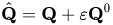
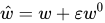
In terms of dual quaternions and the homogeneous coordinates of a point ${\displaystyle {\textbf {P}}:(P_{1},P_{2},P_{3},P_{4})}$ of the object, the transformation equation in terms of quaternions is given by (see ^[7] for details)

${\displaystyle {\tilde {\textbf {P}}}={\textbf {Q}}{\textbf {P}}{\textbf {Q}}^{\ast }+P_{4}[({\textbf {Q}}^{0}){\textbf {Q}}^{\ast }-{\textbf {Q}}({\textbf {Q}}^{0})^{\ast }],}$ where ${\displaystyle {\textbf {Q}}^{\ast }}$ and ${\displaystyle ({\textbf {Q}}^{0})^{\ast }}$ are conjugates of ${\displaystyle {\textbf {Q}}}$ and ${\displaystyle {\textbf {Q}}^{0}}$, respectively and ${\displaystyle {\tilde {\textbf {P}}}}$ denotes homogeneous coordinates of the point after the displacement.

Given a set of unit dual quaternions and dual weights ${\displaystyle {\hat {\textbf {q}}}_{i},{\hat {w}}_{i};i=0...n}$ respectively, the following represents a rational Bezier curve in the space of dual quaternions.

${\displaystyle {\hat {\textbf {Q}}}(t)=\sum \limits _{i=0}^{n}{B_{i}^{n}(t){\hat {\textbf {Q}}}_{i}}=\sum \limits _{i=0}^{n}{B_{i}^{n}(t){\hat {w}}_{i}{\hat {\textbf {q}}}_{i}}}$

where ${\displaystyle B_{i}^{n}(t)}$ are the Bernstein polynomials. The Bezier dual quaternion curve given by above equation defines a rational Bezier motion of degree ${\displaystyle 2n}$.

Similarly, a B-spline dual quaternion curve, which defines a NURBS motion of degree ${\displaystyle 2p}$, is given by,

${\displaystyle {\hat {\textbf {Q}}}(t)=\sum \limits _{i=0}^{n}{N_{i,p}(t){\hat {\textbf {Q}}}_{i}}=\sum \limits _{i=0}^{n}{N_{i,p}(t){\hat {w}}_{i}{\hat {\textbf {q}}}_{i}}}$

where ${\displaystyle N_{i,p}(t)}$ are the ${\displaystyle p}$th-degree B-spline basis functions.

A representation for the rational Bezier motion and rational B-spline motion in the Cartesian space can be obtained by substituting either of the above two preceding expressions for ${\displaystyle {\hat {\textbf {Q}}}(t)}$ in the equation for point transform. In what follows, we deal with the case of rational Bezier motion. The, the trajectory of a point undergoing rational Bezier motion is given by,

${\displaystyle {\tilde {\textbf {P}}}^{2n}(t)=[H^{2n}(t)]{\textbf {P}},}$

${\displaystyle H^{2n}(t)]=\sum \limits _{k=0}^{2n}{B_{k}^{2n}(t)[H_{k}]},}$

where ${\displaystyle [H^{2n}(t)]}$ is the matrix representation of the rational Bezier motion of degree ${\displaystyle 2n}$ in Cartesian space. The following matrices ${\displaystyle [H_{k}]}$ (also referred to as Bezier Control Matrices) define the affine control structure of the motion:

${\displaystyle [H_{k}]={\frac {1}{C_{k}^{2n}}}\sum \limits _{i+j=k}{C_{i}^{n}C_{j}^{n}w_{i}w_{j}[H_{ij}^{\ast }]},}$

where ${\displaystyle [H_{ij}^{\ast }]=[H_{i}^{+}][H_{j}^{-}]+[H_{j}^{-}][H_{i}^{0+}]-[H_{i}^{+}][H_{j}^{0-}]+(\alpha _{i}-\alpha _{j})[H_{j}^{-}][Q_{i}^{+}]}$.

In the above equations, ${\displaystyle C_{i}^{n}}$ and ${\displaystyle C_{j}^{n}}$ are binomial coefficients and ${\displaystyle \alpha _{i}=w_{i}^{0}/w_{i},\alpha _{j}=w_{j}^{0}/w_{j}}$ are the weight ratios and

${\displaystyle [H_{j}^{-}]=\left[{\begin{array}{rrrr}q_{j,4}&-q_{j,3}&q_{j,2}&-q_{j,1}\\q_{j,3}&q_{j,4}&-q_{j,1}&-q_{j,2}\\-q_{j,2}&q_{j,1}&q_{j,4}&-q_{j,3}\\q_{j,1}&q_{j,2}&q_{j,3}&q_{j,4}\\\end{array}}\right],}$

${\displaystyle [Q_{i}^{+}]=\left[{\begin{array}{rrrr}0&0&0&q_{i,1}\\0&0&0&q_{i,2}\\0&0&0&q_{i,3}\\0&0&0&q_{i,4}\\\end{array}}\right],}$

${\displaystyle [H_{i}^{0+}]=\left[{\begin{array}{rrrr}0&0&0&q_{i,1}^{0}\\0&0&0&q_{i,2}^{0}\\0&0&0&q_{i,3}^{0}\\0&0&0&q_{i,4}^{0}\\\end{array}}\right],}$

${\displaystyle [H_{j}^{0-}]=\left[{\begin{array}{rrrr}0&0&0&-q_{j,1}^{0}\\0&0&0&-q_{j,2}^{0}\\0&0&0&-q_{j,3}^{0}\\0&0&0&q_{j,4}^{0}\\\end{array}}\right],}$

${\displaystyle [H_{i}^{+}]=\left[{\begin{array}{rrrr}q_{i,4}&-q_{i,3}&q_{i,2}&q_{i,1}\\q_{i,3}&q_{i,4}&-q_{i,1}&q_{i,2}\\-q_{i,2}&q_{i,1}&q_{i,4}&q_{i,3}\\-q_{i,1}&-q_{i,2}&-q_{i,3}&q_{i,4}\\\end{array}}\right].}$

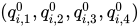
In above matrices, ${\displaystyle (q_{i,1},q_{i,2},q_{i,3},q_{i,4})}$ are four components of the real part ${\displaystyle ({\textbf {q}}_{i})}$ and ${\displaystyle (q_{i,1}^{0},q_{i,2}^{0},q_{i,3}^{0},q_{i,4}^{0})}$ are four components of the dual part${\displaystyle ({\textbf {q}}_{i}^{0})}$ of the unit dual quaternion ${\displaystyle ({\hat {\textbf {q}}}_{i})}$.

• Computational Design Kinematics Lab
• Robotics and Spatial Systems Laboratory (RASSL)
• Robotics and Automation Laboratory

• Quaternion and Dual Quaternion
• NURBS
• Computer Animation
• Robotics
• Robot Kinematics
• Computational Geometry
• CNC machining
• Mechanism Design

References

- ^ McCarthy, J. M. (1990), MIT Press Cambridge, MA, USA
{{citation}}: Missing or empty|title=(help) - ^ Ge, Q. J.; Ravani, B. (1994). "Computer Aided Geometric Design of Motion Interpolants". Journal of mechanical design(1990). 116 (3): 756–762. doi:10.1115/1.2919447.
{{cite journal}}: CS1 maint: multiple names: authors list (link) - ^ Ge, Q. J.; Ravani, B. (1994). "Geometric Construction of Bézier Motions". Journal of mechanical design(1990). 116 (3): 749–755. doi:10.1115/1.2919446.
{{cite journal}}: CS1 maint: multiple names: authors list (link) - ^ Shoemake, K. (1985). "Animating rotation with quaternion curves". Proceedings of the 12th annual conference on Computer graphics and interactive techniques: 245–254. doi:10.1145/325334.325242.
- ^ Bottema, O.; Roth, B. (1990), Dover Pubns http://books.google.co.uk/books?hl=en
{{citation}}: Missing or empty|title=(help)CS1 maint: multiple names: authors list (link) - ^ Roschel, O. (1998). "Rational motion design—a survey". Computer-Aided Design. 30 (3): 169–178. doi:10.1016/S0010-4485(97)00056-0.
- ^ a b Purwar, A.; Ge, Q. J. (2005). "On the effect of dual weights in computer aided design of rational motions". ASME Journal of Mechanical Design. 127 (5): 967–972. doi:10.1115/1.1906263.
{{cite journal}}: CS1 maint: multiple names: authors list (link) Cite error: The named reference "Purwar2005" was defined multiple times with different content (see the help page).
External links